In a previous post, I looked at the overall value of forwards, defensemen, and goaltenders in the context of all players on NHL full strength rosters. That initial assessment was based solely on player impact, yet there are other considerations in a salary cap league. In this post, we’ll look at two major factors that modify player value.
Definitions
I covered these definitions in the last post. They are key to understanding the rest of the post, so I’ll re-hash them here. If you’re still familiar with them, feel free to jump ahead to the next section.
- Impact: The calculated 5v5 Net Goals/60 Above Replacement for a player. Replacement is defined as a 25th percentile player based on historical data. We look at only the 5v5 Impact to put all players on equal footing for comparison. Since roughly 80% of NHL game time is spent at 5v5, it gives us a good picture of how a player will impact team performance. It also allows us to utilize the largest sample size of time on ice to based projections on.
- Cap Hit: The actual cost for a player, in cap dollars, which represents the actual cost for a team to employ a player on their roster. It may be different than the actual salary based on the contract structure, however the cap hit gives us the best measure of player cost relative to the constraints of the salary cap.
- Value: The overall impact of the player, expressed in cap dollars, in the context of the complete set of players on NHL full strength rosters. The conversion from impact to cap dollars is calculated using best fit curves on all active contracts for players on full strength rosters. This gives us a relative measure of how efficiently cap space is being spent on each player with consideration for their relative impacts. When combined at the team level, it gives us a picture of how efficiently a team is spending cap space throughout their entire roster. We’ll look at these curves momentarily.
- Market Value: The impact of the player, expressed in cap dollars, in the context of the players who signed their current contract within the past 2 calendar years. A curve similar to the Value curve is used, with only the applicable contracts used for fitting. This give us a measure of how much cap space teams are currently paying for players based on player Impact.
Value of RFAs
There are three main types of contracts that we see in the NHL, based on the player’s status when they sign their deal:
- Entry-Level Contracts (ELC): These deals are the first a player signs with an NHL club. There are heavy restrictions regarding the maximum salary a team can offer.
- Restricted Free Agents (RFA): These players were previously under contract with an NHL team and their current team still owns their signing rights. It’s possible for other teams to sign them via an offer sheet but they will have give up draft picks if they are successful in acquiring the player.
- Unrestricted Free Agents (UFA): These players are free to sign with any team, no strings attached.
We’re going to break down recent contracts by these three groups to get a more detailed picture of market value. We expect to see a small number of ELCs since most players that play in the NHL on an entry level deal do so a couple of seasons after signing. We also expect to see them scattered near the league minimum cap hit due to the restrictions for ELCs.
UFA and RFA contracts should be more interesting. Given teams have more leverage with RFAs, we may see the market value for RFAs below that for UFAs. Given RFAs are typically in their early-mid 20s, they are still developing or entering their prime. That is often not the case for UFAs and it may affect the market value rates as well.
Let’s dig in.
Forwards
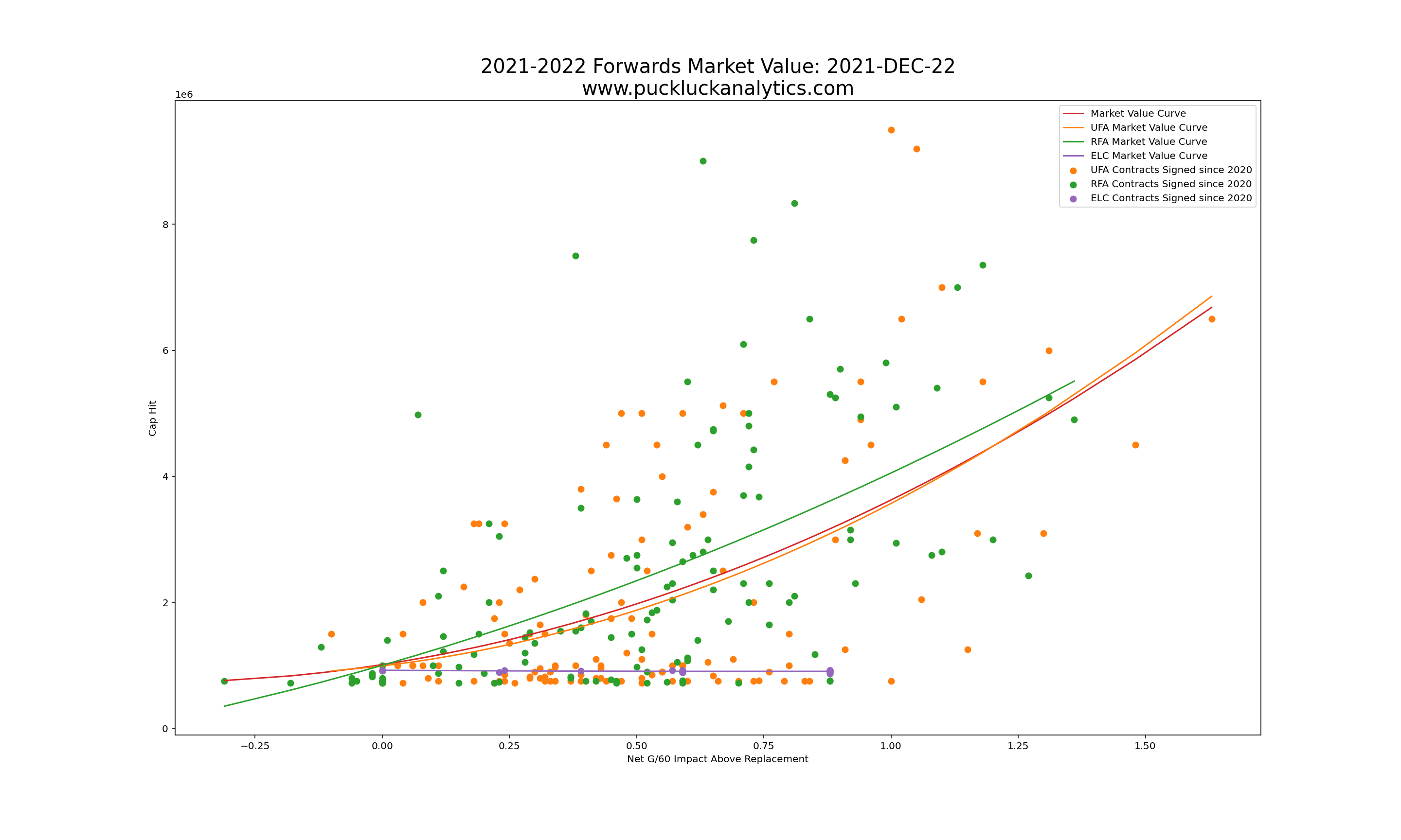
It’s intriguing that the UFA curve for forwards follows the overall curve closely, while the RFA curve sits higher. This runs counter to the thought that teams have more leverage with RFAs, allowing them to keep cap hits lower. Likely, the fact that RFAs are younger and still developing is driving this. Teams want to lock up their young players to take advantage of their potential over the long term.
A few observations for the forwards group:
- The market rate for RFAs is higher than UFAs, although not by a large amount. The biggest discrepancy is for players with Impact in the middle of the full range. One possibility is that teams are over-valuing the potential their mid-grade prospects.
- Signing UFAs appears to be a good strategy for filling holes in the roster, particularly in depth positions. The Market Value is slightly lower than it is for RFAs. There are also plenty of contracts near the league minimum with moderate Impact, providing opportunity to find high value deals.
- ELCs are an infrequent, but highly effective method of obtaining extremely high value contracts. Since the maximum cap hit is set, players with even moderate impact provide excellent value. Getting players still on ELCs into the NHL is a worthwhile objective.
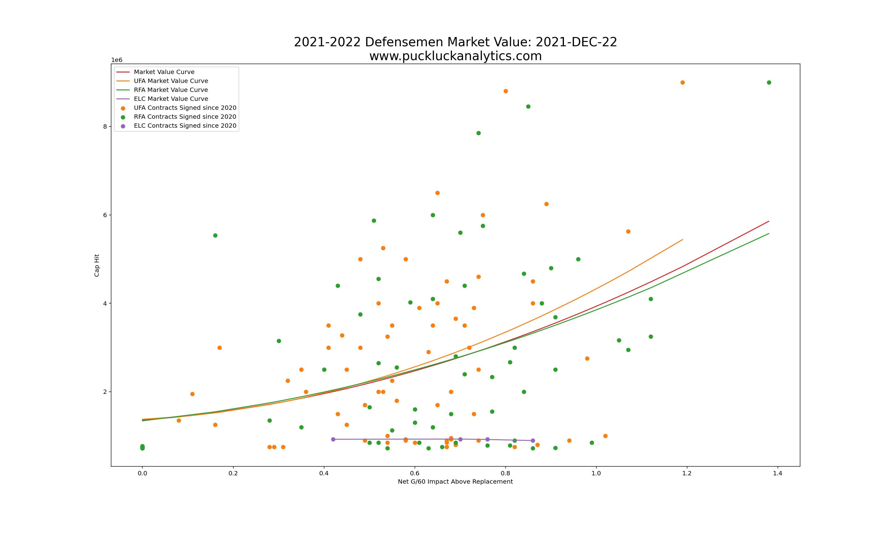
Defensemen
Unlike the curves for forwards, the curves for defensemen show a market curve for UFAs that is above the RFA curve. This time, the RFA curve follows the overall curve more closely, however the UFA is quite close as well and mainly deviates at high Impact.
Observations for the defense group:
- The market rate for UFAs is higher than the market rate for RFAs for mid to high Impact players. Using UFAs to fill holes in the top of the defense corps appears to be an inefficient method of using cap space.
- There are a handful of both UFA and RFA contracts near the league minimum cap hit with widely varying impacts. It’s possible to find high value deals in both groups.
- As with the forwards, ELCs are an excellent method of finding high value contracts but they are less common.
Goaltenders
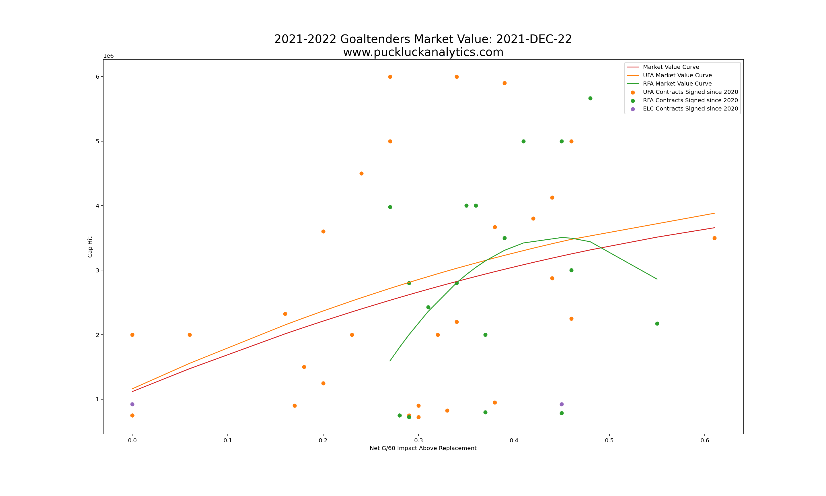
We see some oddities with the goaltender curves due to the small number of data points. The UFA curve actually follows the overall curve quite closely, but the RFA curve is bent in a strange manner due to the small number of data points and there aren’t enough ELCs to fit a curve.
Observations for goaltenders:
- The curve for UFAs follows the overall curve, bent the opposite way than we would likely expect. There seems to be a general trend of over-paying for mid-impact goalies.
- The RFA curve is clearly exaggerated due to a small number of data points. It shows the same trend as the UFA curve, however, with mid-level goalies getting the highest cap hits.
- While we can’t fit the curve for ELCs due to limited data points, there is still potential to find a high value contract this way.
Value Modifier: RFA on Expiry
From the curves above, we can determine the difference in market value for a player based on their contract expiry status. By setting the default method of filling a roster spot as signing a UFA, we can obtain a value for pending RFAs.
The value of a player who will become an RFA upon contract expiry will be equal to their value as determined in the previous post assessing player value, with an adjustment for the difference in expected signing cost for an RFA relative to a UFA. This may be a positive or negative adjustment, as we saw from the difference in the curves between forwards and defensemen.
Value of Cap Space
The second player value modifier we’ll consider relates to the value of cap space. Opportunity cost is a concept from economics that represents the potential benefits that one misses out on when choosing one alternative over another. We’ll use the concept to understand the value of an efficient (or inefficient) contract.
Since there are many methods of acquiring a player, such as through free agency or trade, we want to consider overall value. That leads us to using the overall value curve from the first post in this series. For roster construction, the opportunity cost is the difference between the player’s cap hit and the league average cap hit for a player of their impact, as defined by the value curves.
Example – Bear / Foegele trade
Let’s put the concepts from these two posts on player value to practical use by using it to evaluate a one-for-one trade. One of the trades I checked in on this season was the deal that sent Ethan Bear to Carolina and Warren Foegele to Edmonton. Based on projected player impacts, Carolina had the initial upper hand. However, we now have two additional factors to consider that could change the assessment.
Player Value: Based on each player’s projected Impact, their projected value is calculated as the cap hit at the point on the overall value curve that corresponds to their impact. Bear’s projected Impact is 0.84 Net G/60 Above Replacement, which translates to a value of $4.4M while Foegele’s Impact of 0.61 translates to a value of $2.99M. This is essentially the assessment we made in the initial look at the trade when we only considered player impact. If we stop here, the Hurricanes won the trade, getting a total value roughly 150% of what they gave up.
Contract Expiry Value: We assumed that a player on an expiring contract would be replaced by a UFA by default. Since Foegele will be a UFA on expiry, there is no modification to his value. Bear, on the other hand will be an RFA when his contract is up so his next contract will be at the RFA market rate rather than the UFA market rate. To get the value, we calculate the market rate for UFAs and RFAs at Bear’s projected Impact and find the difference. Based on the difference in the curves, we can expect that Bear can be signed for $275k less than a UFA defensemen with the same Impact.
Cap Efficiency Opportunity Cost: The opportunity cost is the difference between the player value and cap hit. Bear has a cap hit of $2M, so we simply subtract that cap hit from the player value we calculated above. In Bear’s case, we get +$2.4M. In other words, the Hurricanes are getting more value from Bear than they are paying for, leaving them an additional $2.4M of cap space that they can spend elsewhere. Since Foegele was an unsigned RFA at the time of the trade, our assumption here is that the Oilers would sign him at his current value. Signing him for more or less is a separate transaction that should be judged on it’s own merit (for the record, Edmonton subsequently signed him for $2.75M which is slightly below his projected value).
| Ethan Bear (to CAR) | Warren Foegele (to EDM) | |
| Projected Value | $4,421,000 | $2,989,000 |
| Contract Expiry Value | $275,190 | $0 |
| Cap Efficiency Opportunity Cost | $2,421,000 | $0 (Unsigned RFA at time of trade) *($239,000 based on contract signed after the trade) |
| Total Player Value | $7,117,190 | $2,989,000 |
When we add it all up, we get a fairly different picture than the original assessment of the trade that was based on projected Impact alone. While it still looks like Carolina won the trade, it now appears they managed to get 240% value back for what they gave up. It’s a significant increase from the 150% based only on Impact.
What’s Next?
Now that we have a handle on assessing player value, we need to complete the value picture by looking at prospects and picks. Stay tuned for the third post in this series where we’ll tackle future assets and put the whole picture together.